There was a recent tweet in the crypto-Twitter sphere (can’t seem to find now) which discussed constant-mix – a well known, albeit simplistic, dynamic portfolio management technique – in the context of Uniswap and impermanent loss. What surprised me about that thread is that people seemed unaware of constant-mix. The matter of the fact is that constant-mix has been known and used since 1985, potentially much earlier. Yep, you read that right! There’s awesome journals from Perold et. al on this topic since back then. In fact, part of this post will be from those papers.

Here, I wanted to take the time to discuss portfolio management strategies through the lens of Uniswap. What’s interesting about Uniswap, and which people don’t seem to realize, is that it isn’t an exchange! Well, at the very least, the exchange side of things is a second order effect. Instead, it is a smart contract that implements a very specific type of dynamic portfolio management strategy known as constant-mix, which reduces to “buy tokens as they fall, sell as they rise”. This – in turn – has a concave payout structure. We’ll go into all of this shortly.

If, however, someone insists that Uniswap is an exchange, then while that person would technically be right, it would still be a fact that Uniswap is an exchange only through a second-order effect. It’s like saying that mayo can be used as food. True, it can, but that’s really a second-order effect of consuming mayo, and it should primarily just be used for its intended purpose: a condiment.

The goal, left for me to achieve, is to explain everything in the simplest possible terms, making it available even to the laypeople. Lots of people in crypto tend to reinvent basic things known for decades, including impermanent loss, automated market makers, and more. In this post, we’ll make it all pretty simple. But not simpler.

Background

First of all, in the rest of this post I’m going to ask for you to forget the terms “impermanent loss” or “automated market makers” or whatever else comes tied to Uniswap. It’s all – quite literally – a confusing reinvention of things that already exist. We’ll try to learn these things through proper terms such that you can go on your merry way and independently read the appropriate literature from the finance world and not have to rely on bad crypto blog posts … like this one.

Now, let’s get started. In order to understand why Uniswap does what it does, let’s first state our goal: we want to understand how Alice, a savvy investor, can distribute her assets between stocks and cash in a way that’s optimal for her risk profile. The marker behavior will – of course – inform her risk profile to a certain extent.

For simplicity, Alice can only either keep her assets in cash or can buy stock. In other words, Alice needs to decide how to “balance” and “rebalance” her portfolio between these two assets. This already looks like a pool in Uniswap. We enforce this simplifying restriction because we can reason about the total value of Alice’s assets through a single-dimensional variable, i.e. the stock value. Cash remains constant. If we were to use two assets, such as stocks and bonds, we’d need to work on visualizing three dimensional surfaces. Not too bad, but let’s make it easier on us, and worry just about a single input variable, x (the stock value), and its relationship to y (the total portfolio value denominated in USD). All analysis here trivially extends to any number of variables.

If Alice is highly risk-averse, she’ll choose to go all in on cash. If she’s more risk-prone, she’ll go into stock. Notice, however, that I am not asking several questions, including “which stocks should Alice buy?”. This is an irrelevant question in the context of portfolio management. Instead what matters for Alice is “when she should buy or sell stock” and “how much”.

In rest of this post, we’ll discuss three strategies:

• Buy-and-hold: do nothing;
• Constant-mix: buy stocks as they fall, sell as they rise;
• Constant-proportion portfolio insurance (CPPI): sell stocks as they fall, buy as they rise;

The interesting thing between the three is that they will have different payouts based on the way the market behaves over time. The first will have a linear payout, meaning that long-term payout is only dependent on the current market condition (i.e. how well stocks are doing), whereas the latter will have concave and convex payouts, meaning that the second will do well if there’s reversions to the mean (i.e. maxima of concave is in the middle), whereas the third will do well if there’s displacement from the mean (i.e. the maxima is if the stocks rally or fall extensively). We’ll describe all of these in more details in just a bit.

Portfolio Strategy #1: Buy and hold; or, do nothing.

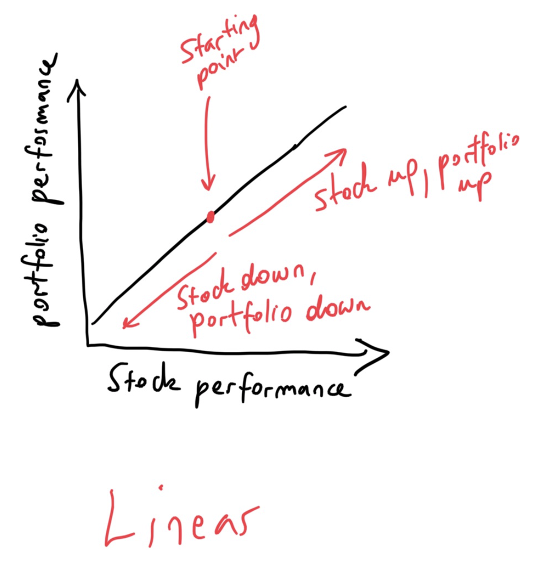
Do nothing, or typically referred to as a “buy-and-hold” strategies are pretty much what they sound. Alice, at the beginning, chooses a certain allocation of cash / stock, and then rides it out. The better the stock, the better the portfolio outcome, as shown in the picture above. The net payout is – obviously – a linear function whose slope is dependent on the original allocation between stock and cash. The more stock, the higher the slope, as shown below.

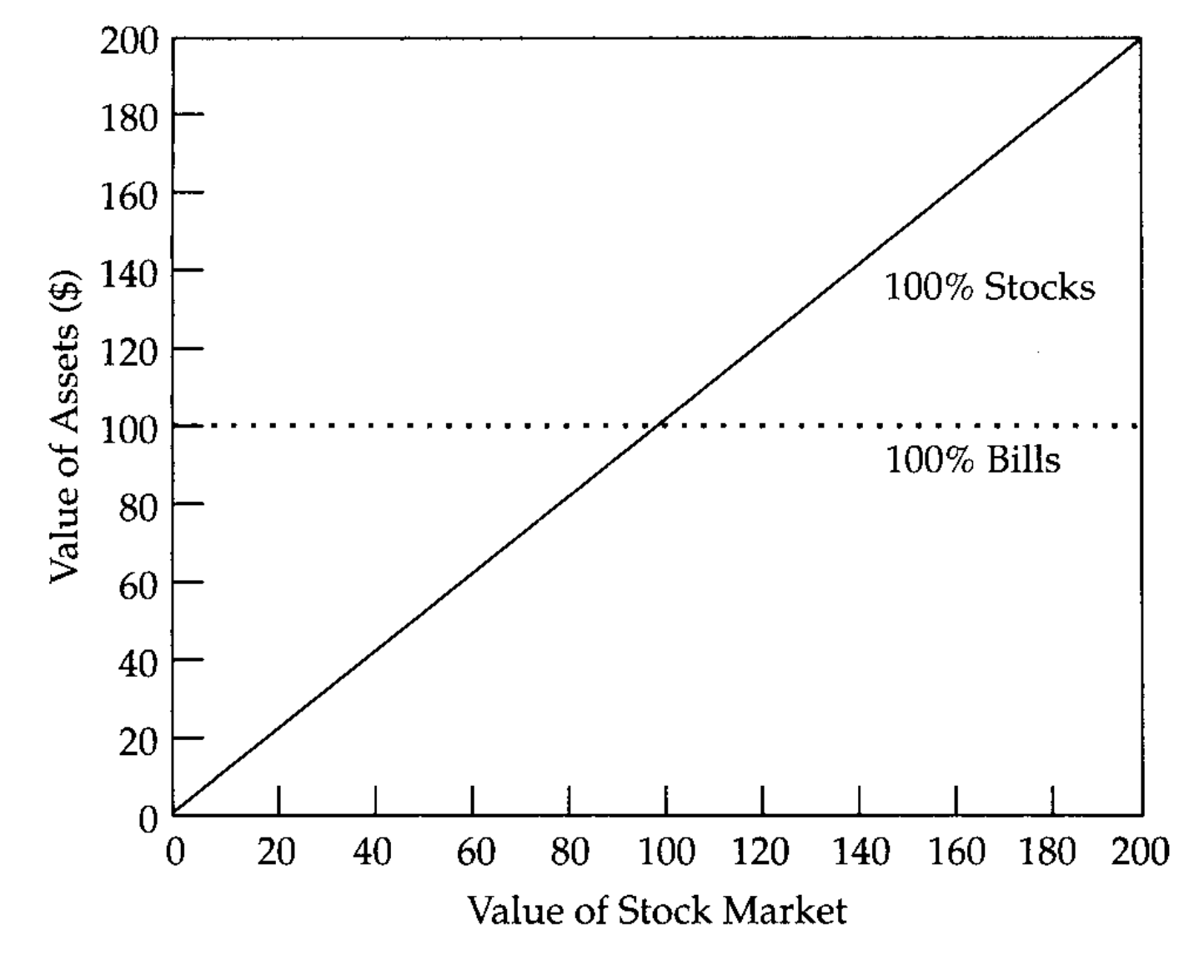
When Alice is all in on cash, her net portfolio performance is independent of the stock performance. Slope would be zero. Pretty straightforward.

Portfolio Strategy #2: Constant-mix; or, buy stocks as they fall, sell as they rise.

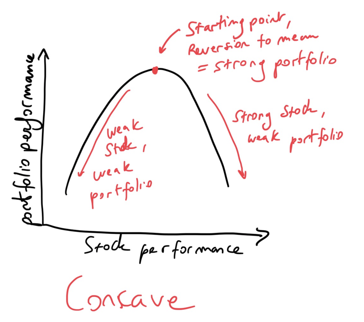
This is when strategies get a bit more interesting. By definition, these strategies aim to maintain an exposure to stock that is constant in proportion to the portfolio wealth. This is exactly how Uniswap works. After creating a new pool, the protocol aims to maintain a constant proportion between two assets \(y\) and \(x\) (i.e. \(xy = k\), for some constant \(k\)).

Conceptually speaking, constant-mix strategies aim to increase exposure to an asset as its value is decreasing. Here’s the classic example in terms of stock-to-bills. Suppose Alice puts $60 in stocks and $40 in cash, thus establishing a 60/40 constant mix pool. Assume the stock declines by 10%, thus reducing stock value from $60 to $54, and portfolio value from $100 down to $94. At this point, the proportion will be $54/$94, or 57.4%, which is below the desired 60% of the pool. At this point, the protocol dictates that Alice must buy more stock (since she needs to buy the asset that depreciating), and thus increase her stock exposure back up to the 60% mark. Alice will need to purchase $2.40 of stock from her cash position, thus bringing stock to $56.40, and reducing cash position down to $37.60. The new percentages are then again 60/40 (i.e. 56.4/94 = 60; 37.6/94 = 40). Let me reiterate: this is identical to how a Uniswap pool works, with the caveat that anyone can deposit into a specific token-pair pool, instead of just Alice. However, instead of there being stocks and bills, there’s a constant proportion between – say – AVAX and ETH.

Now, let’s be clear about one thing: this is weird. Why would Alice, a savvy investor, be buying more of asset that depreciating in value. The answer, naturally, is not because Alice is uninformed. On the contrary, it is because Alice believes that the market she’s implementing this strategy is volatile and mean-reverting. If that’s the case, of course, then it makes sense for Alice to keep buying more of the asset that’s depreciating because it will soon revert back to higher values, and she’d be getting them for a steal! Under these conditions, it doesn’t matter how much an asset drops, you just keep buying.

Constant-mix strategies (i.e. Uniswap) are profitable in volatile – but mean-reverting – markets.

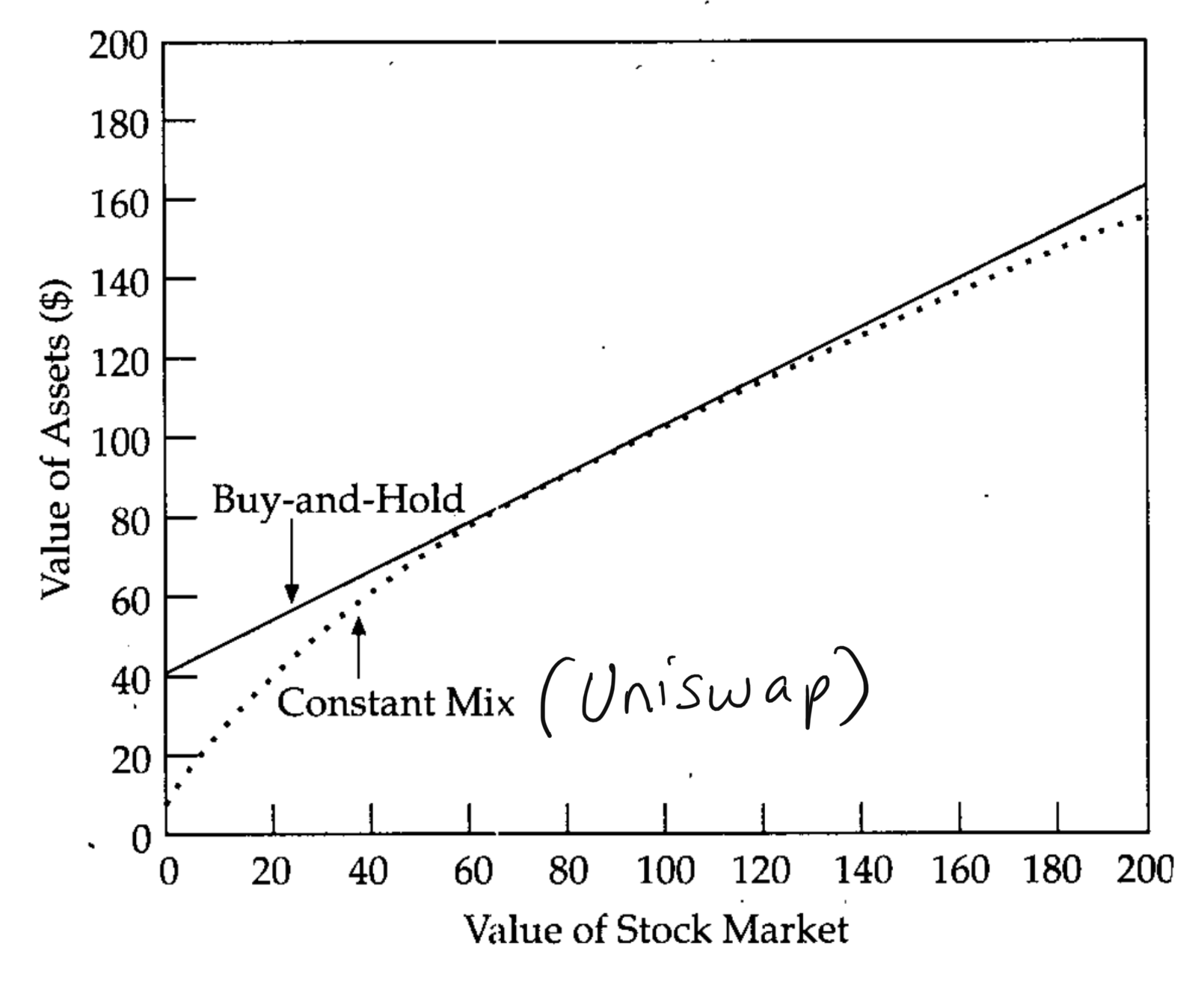
Since Uniswap is just a constant-mix market, it means that it’s always profitable to be a liquidity provider as long as the target pool includes only mean-reverting markets. If – on other hand – you provide liquidity to markets that diverge wildly (i.e. perpetually depreciate or perpetually appreciate), then participating as an LP into Uniswap is strictly less profitable than – quite literally – just a buy-and-hold strategy. Or, as we shall soon see, CPPI’s. The figure below shows constant-mix vs buy-and-hold.

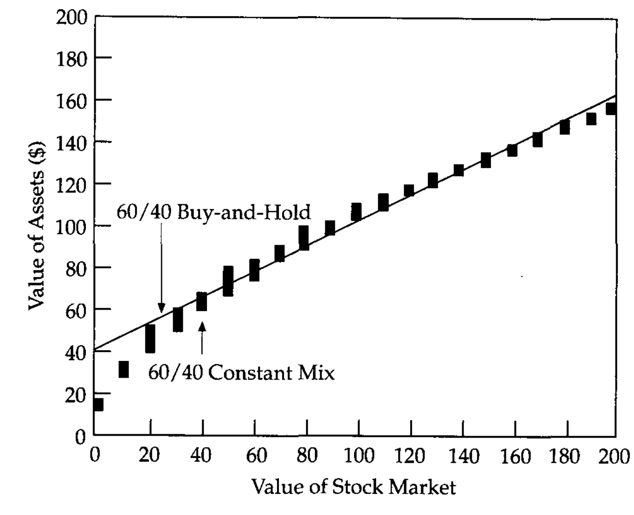
This effect is also show more precisely in the figure below. As one can see, constant-mix is strictly less-profitable in the long-run if you just buy-and-hold under markets that diverge. Why? Scenario 1: if the stock market is going down in value dramatically (and staying there), then constant-mix is buying more and more of worthless assets. Scenario 2: if the stock market is going up in value dramatically (and staying there), then constant-mix is selling more and more of the stock in preference of the depreciating value of the other asset (in this case, cash).

So, in summary, being an LP in Uniswap pays if the assets revert back to the usual mean. Otherwise, it’s strictly a loss, and not a recommended strategy for Alice.

Portfolio Strategy #3: Constant-proportion portfolio insurance (CPPI); or, sell stocks as they fall, buy as they rise.

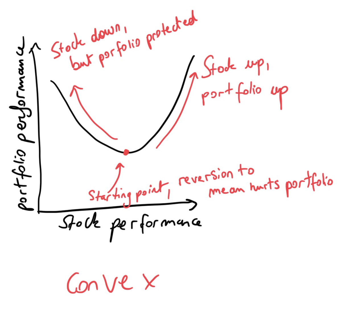
What happens if the markets aren’t mean-reverting? Instead, what if the markets divert widely from the entry point, i.e. depreciate or appreciate greatly. Naturally, as outlined above, it isn’t optimal for Alice to implement a constant-mix strategy (i.e. be a Uniswap LP). Instead, Alice should sell assets as they depreciate and buy those are appreciate. This makes sense: if Alice knows that stocks will keep depreciating, she should sell off as much as she can; if instead she knows that stocks will keep appreciating, she should buy off as much as she can. These types of strategies, known as CPPIs, take the form of: dollars in stock = \(m\)(Assets - Floor); Here, \(m\), is a fixed multiplier, part of Alice’s risk tolerance. As the figure above represents, these strategies perform well on divergence, rather than reversion, thus making them convex.

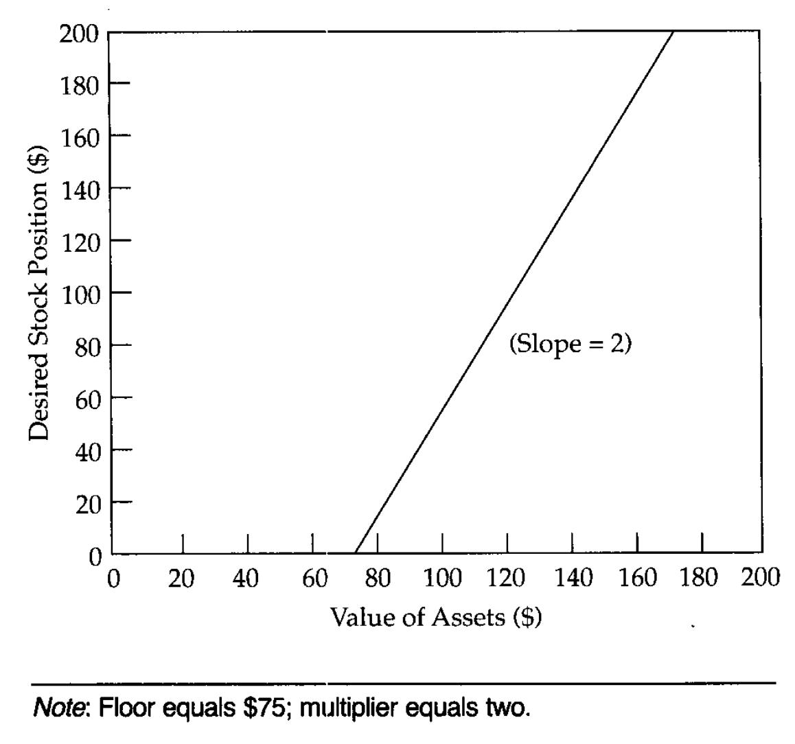
Here’s how CPPI works. Suppose Alice chooses \(m = 2\), and a floor of $75. The latter is Alice’s lower-bound tolerance to the loss through total stock depreciation. Given these numbers, Alice’s dollars in stock = \(2\)*($100 - $75) = $50. Therefore, Alice will split her portfolio 50/50 between stock and cash. The figure below represents the diagram for this risk profile:

Given Alice’s choice of \(m = 2\) and a floor of $75, here’s how her portfolio will behave on a downturn. Suppose the stock falls 10%, depreciating her stock from $50 to $45, and total portfolio from $100 to $95. Since the CPPI rule enforces a stock position off \(2*($95-$75) = $40\), Alice must sell an additional $5 worth of stock and reduce her exposure down further. In other words, a 10% downturn in stock forced Alice to sell $5 worth of her stock. She is now “lighter” in her riskier asset.

CPPI strategies outperform constant-mix (i.e. Uniswap) in diverging (depreciating or appreciating) markets.

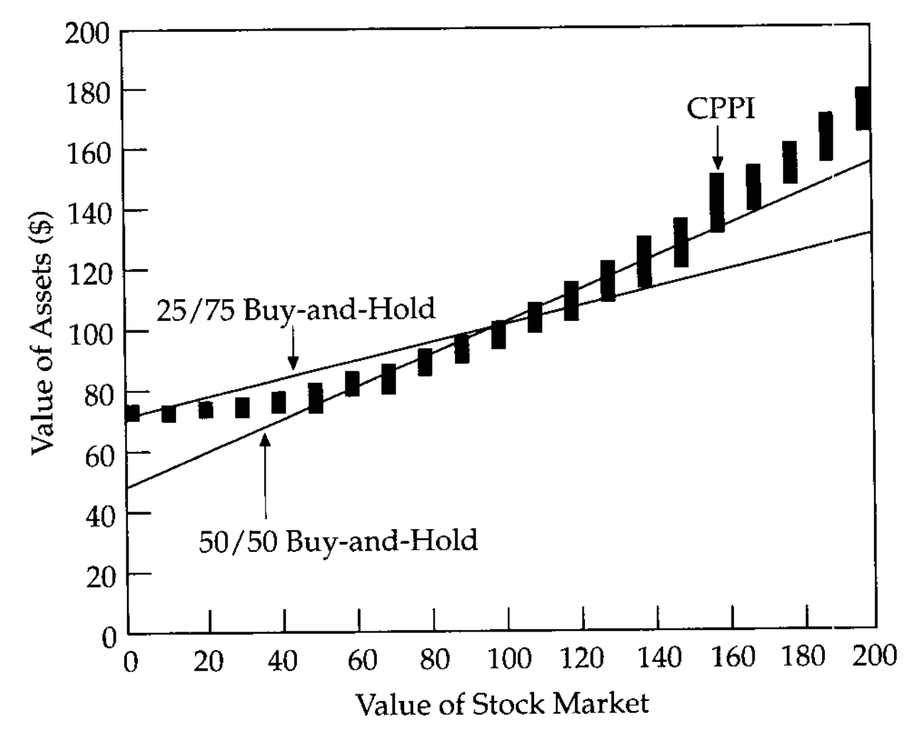
Under CPPI, the portfolio will naturally do at least as well as the floor. In a roundabout way, CPPI implements options over stocks, without using standard options techniques. Alice’s loss is capped at a total of $25 (since her floor is $75), while also exposing herself to high upside (albeit not unlimited). In summary, in bear markets CPPI will protect Alice and in bull ones it will do very well. However, it will under-perform constant-mix (i.e. Uniswap) if there are frequent reversals. The graph below shows CPPI vs two different buy-and-hold strategies.

Final thoughts

Uniswap is an interesting experiment. It is one of the first wide-scale successful deployments of basic constant-mix smart-contract-based portfolio management between any two pairs of ERC-20s on Ethereum. The second-order effect is exchange functionality, although it can be argued decisively that exchanging assets through this method is widely subpar to standard orderbook-based exchanges. Please do not @ me on Twitter about this, I have read the arguments on AMMs and they are factually, blatantly wrong. So awfully wrong. There’s a reason why AMMs aren’t used in every single mainstream financial market.

In any case, what’s going to be interesting is to see some on-chain protocols that provide CPPI strategies. It will be quite interesting to then see how those play out with constant-mix ones. I would expect traders to recalibrate their positions into Uniswap and CPPISwap quite frequently depending on market conditions. What is obvious, however, is that we’re so early. Many of these are yet to be implemented.

References

1. Perold, Andre and Sharpe, William. Dynamic Strategies for Asset Allocation. Accessed 2020.